Tuesday, September 23, 2014

Today we will discuss about the Design Pattern: Model-View-Controller, which is also very famous by its abbriviation MVC. By definition, MVC is to isolate the business logic from the User Interface which gives great degree of flexibility to change business logic independently to the user interface and vice versa.

Basics of MVC

In MVC, User Interface acts as the View; Business logic acts as the Model and the link which provides the link between the View and Model is known as the Controller. In real time business, MVC is used anywhere, where users have a choice to select his or her view. For example, Windows Media Player, Gmail or Yahoo mail and so on. All these type of application provides us the option to select the skin as per our choice.

Let’s take an example: We have to develop one Sales report for our corporate intranet. This report must have the option to display the sales data in the classical report format; different charts – pie, bar, line or both – report & chart and it must be based on the User’s choice. This type of requirements where we can easily separate the Business logic and the views are the best candidates for MVC.
Generally, Model sends the data to controller and controller will pass that data to Views and views will display the data as per their nature. In SAP, our business logic(model) will not send data unless and until View request for an data because ABAP is event driven language. Like user has to run some transaction to get the data, means application view has to initiate the process and ask for the data from the Model. In this requesting process, Controller will help the view to be apart from the model.

UML for MVC

UML diagram of the typical MVC application would be:

As we can see here, Model will send the data to the Controller and controller will pass that information to the View. Now, its a view’s responsibility to create a user specific view – Report, or Chart.

Advantages of using MVC:

Since both our business logic and view logic are different, we can easily change any of the logic without interrupting the other part.
In the next post, we will see how we can implement the MVC design pattern in ABAP usin the ABAP Objects.

Demo Application

To implement the MVC, we will create two applications – One will generate an output in ALV and other will generate an output Smartforms. We will put our business logic in the MODEL class. We will create one CONTROL class to establish control between Model and Views.

Our business logic for this example is fairly simple – select the Sales Orders from the VBAK which were created in last ten days. The public method GET_DATA in the class ZCL_MODEL will act as the business logic. Additionally, this class has the public attribute T_VBAK which will be set by the GET_DATA and hold our data from the table.

UML

The UML diagram for any of the application would be like:

Model Class Setup

Model Method Definition

Model Attribute definition

Code Snippet of method GET_DATA
This code would be implemented in the method GET_DATA

 
* Parameters
* Importing IR_ERDAT TYPE TPMY_R_DATE Ranges for date
*
METHOD get_data.
*
* Get data and save into attribute T_VBAK
  SELECT * FROM vbak
         INTO  TABLE t_vbak
         WHERE erdat IN ir_erdat.
*
*
ENDMETHOD.

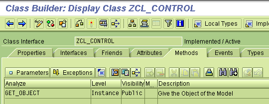
Controller Class Setup

Our controller class ZCL_CONTROL will have a method GET_OBJECT which will give us an object of the model class. We require a public attribute which can refer to the object created in the method GET_OBJECT.
Controller Method definition:

Controller Attributes definition:

Code Snippet for method GET_OBJECT:

 
* Parameters
* Importing IF_NAME TYPE CHAR30 Model class name
*
METHOD get_object .
*
  DATA: lo_object TYPE REF TO object.
*
* Generic object reference to importing class
  CREATE OBJECT lo_object TYPE (if_name).
  IF sy-subrc = 0.
*   Downcasting to assign generic object to O_MODEL
    o_model ?= lo_object.
  ENDIF.
*
ENDMETHOD.

In the next post we will see, how we will use the controller class in our view and access the business logic encapsulated in Model class.

First Demo Application – ALV

For our first Application view will be ALV output. To get the data for the ALV into the application, we will use the reference of the MODEL class created in the Controller. This way our model class is entrily separated by the view.

Code Snippet for View 1: ALV of MVC design

 
*&---------------------------------------------------------------------*
*& Purpose - ABAP Design Patterns - Model View Controller MVC - ALV demo
*& Author  - Naimesh Patel
*& URL     - http://zevolving.com/?p=52
*&---------------------------------------------------------------------*
*
REPORT  ztest_mvc_alv.
*
START-OF-SELECTION.
*---------
* Controller
*---------
  DATA: lo_control TYPE REF TO zcl_control.
*
* Iniiate controller
  CREATE OBJECT lo_control.
*
* Get the object from Control
  CALL METHOD lo_control->get_object
    EXPORTING
      if_name = 'ZCL_MODEL'.
*
*---------
* Model - Business Logic
*---------
* Date Range
  DATA: r_erdat  TYPE RANGE OF vbak-erdat,
        la_erdat LIKE LINE OF r_erdat.
*
  la_erdat-sign = 'I'.
  la_erdat-option = 'BT'.
  la_erdat-low = sy-datum - 10.
  la_erdat-high = sy-datum.
  APPEND la_erdat TO r_erdat.
*
* Get data method
  CALL METHOD lo_control->o_model->get_data
    EXPORTING
      ir_erdat = r_erdat.
*
*---------
* View - ALV output
*---------
  DATA: lo_alv TYPE REF TO cl_salv_table.
*
  DATA: lx_msg TYPE REF TO cx_salv_msg.
  TRY.
      cl_salv_table=>factory(
        IMPORTING
          r_salv_table = lo_alv
        CHANGING
          t_table      = lo_control->o_model->t_vbak ).
    CATCH cx_salv_msg INTO lx_msg.
  ENDTRY.
*
*
* Displaying the ALV
  lo_alv->display( ).

First Demo Application – SmartForms Output

Our Second application is fairly simple once we have implemented the first application as our core logic of getting the data is out of the report. In this application only part which differs is calling the Smartform.
Code Snippet for View 2: Smartforms of MVC design

 
*&---------------------------------------------------------------------*
*& Purpose - ABAP Design Patterns - Model View Controller MVC - 
*&           SmartForms Demo
*& Author  - Naimesh Patel
*& URL     - http://zevolving.com/?p=52
*&---------------------------------------------------------------------*
*
REPORT  ztest_mvc_view_2_ssf.
*
START-OF-SELECTION.
*---------
* Controller
*---------
  DATA: lo_control TYPE REF TO zcl_control.
*
* Iniiate controller
  CREATE OBJECT lo_control.
*
* Get the object from Control
  CALL METHOD lo_control->get_object
    EXPORTING
      if_name = 'ZCL_MODEL'.
*
*---------
* Model - Business Logic
*---------
* Date Range
  DATA: r_erdat  TYPE RANGE OF vbak-erdat,
        la_erdat LIKE LINE OF r_erdat.
*
  la_erdat-sign = 'I'.
  la_erdat-option = 'BT'.
  la_erdat-low = sy-datum - 10.
  la_erdat-high = sy-datum.
  APPEND la_erdat TO r_erdat.
*
* Get data method
  CALL METHOD lo_control->o_model->get_data
    EXPORTING
      ir_erdat = r_erdat.
*
*---------
* View - Smartform Output
*---------
* Smartform FM
  DATA: l_form TYPE tdsfname VALUE 'ZTEST_MVC_VIEW_2',
        l_fm   TYPE rs38l_fnam.
*
  CALL FUNCTION 'SSF_FUNCTION_MODULE_NAME'
    EXPORTING
      formname           = l_form
    IMPORTING
      fm_name            = l_fm
    EXCEPTIONS
      no_form            = 1
      no_function_module = 2
      OTHERS             = 3.
*
* calling Smartform FM
  DATA: ls_control  TYPE ssfctrlop.  " Controlling info
  DATA: ls_composer TYPE ssfcompop.  " Output info
*
  CALL FUNCTION l_fm
    EXPORTING
      control_parameters = ls_control
      output_options     = ls_composer
      user_settings      = ' '
      t_vbak             = lo_control->o_model->t_vbak
    EXCEPTIONS
      formatting_error   = 1
      internal_error     = 2
      send_error         = 3
      user_canceled      = 4
      OTHERS             = 5.
  IF sy-subrc <> 0.
    MESSAGE ID sy-msgid TYPE sy-msgty NUMBER sy-msgno
            WITH sy-msgv1 sy-msgv2 sy-msgv3 sy-msgv4.
  ENDIF.

Let’s say, in future we enhanced the business logic model class and now we want to implement for the business. In this case, we just have to change the object reference created in the Controller and we are good to go. Obviously, we have to take care of the newly created methods or methods which parameters are enhanced.

Wednesday, September 17, 2014

SAP Security, Roles, Authentication

SAP Security & Roles & Authentication:

https://www.youtube.com/watch?v=9D9e-lNpuk0

The SQL Trace (ST05) – Quick and Easy

the-sql-trace-st05-quick-and-easy

The SQL Trace (ST05) – Quick and Easy

The SQL Trace, which is part of the Performance Trace (transaction ST05), is the most important tool to test the performance of the database. Unfortunately, information on how to use the SQL Trace and especially how to interpret its results is not part of the standard ABAP courses. This weblog tries to give you a quick introduction to the SQL Trace. It shows you how to execute a trace, which is very straightforward. And it tells how you can get a very condensed overview of the results--the SQL statements summary--a feature that many are not so familiar with. The usefulness of this list becomes obvious when the results are interpreted. A short discussion of the ‘database explain’ concludes this introduction to the SQL Trace.

1. Using the SQL Trace

Using the SQL trace is very straightforward:

Call the SQL trace in a second mode
Make sure that your test program was executed at least once, or even better, a few times, to fill the buffers and caches. Only a repeated execution provides reproducible trace results. Initial costs are neglected in our examination
Start the trace
Execute your test program in the first mode
Switch off the trace. Note, that only one SQL trace can be active on an application server, so always switch your trace off immediately after your are finished.
Display the trace results
Interpretation of the results

Note, the trace can also be switched on for a different user.

=> In this section we showed how the SQL trace is executed. The execution is very straightforward and can be performed without any prior knowledge. The interpretation of the results, however, requires some experience. More on the interpretation will come in the next section.

2. Trace Results – The Extended Trace List

When the trace result is displayed the extended trace list comes up. This list shows all executed statements in the order of execution (as extended list it includes also the time stamp). One execution of a statement can result in several lines, one REOPEN and one or several FETCHES. Note that you also have PREPARE and OPEN lines, but you should not see them, because you only need to analyze traces of repeated executions. So, if you see a PREPARE line, then it is better to repeat the measurement, because an initial execution has also other effects, which make an analysis difficult.

If you want to take the quick and easy approach, the extended trace list is much too detailed. To get a good overview you want to see all executions of the same statement aggregated into one line. Such a list is available, and can be called by the menu ‘Trace List -> Summary by SQL Statements’.

=> The extended trace list is the default result of the SQL Trace. It shows a lot of and very detailed information. For an overview it is much more convenient to view an aggregated list of the trace results. This is the Summarized SQL Statements explained in the next section.

3. Trace Results - Summarized SQL Statements

This list contains all the information we need for most performance tuning tasks.

The keys of the list are ‘Obj Name’ (col. 12), i.e. table name, and ‘SQL Statement’ (col. 13). When using the summarized list, keep the following points in mind:

Several coding positions can relate to the same statement:
The statement shown can differ from its Open SQL formulation in ABAP.
The displayed length of the field ‘Statement’ is restricted, but sometimes the displayed text is identical.
In this case, the statements differ in part that is not displayed.

The important measured values are ‘Executions’ (col. 1), ‘Duration’ (col. 3) and ‘Records’ (col. 4). They tell you how often a statement was executed, how much time it needed in total and how many records were selected or changed. For these three columns also the totals are interesting; they are displayed in the last line. The other totals are actually averages, which make them not that interesting.

Three columns are direct problem indicators. These are ‘Identical’ (col. 2), ‘BfTp’ (col. 10), i.e. buffer type, and ‘MinTime/R.’ (col. 8), the minimal time record.

Additional, but less important information is given in the columns, ‘Time/exec’ (col. 5), ‘Rec/exec’ (col. 6), ‘AvgTime/R.’ (col. 7), ‘Length’ (col. 9) and ‘TabType’ (col. 11).

For each line four functions are possible:

The magnifying glass shows the statement details; these are the actual values that were used in the execution. In the summary the values of the last execution are displayed as an example.
The ‘DDIC information’ provides some useful information about the table and has links to further table details and technical settings.
The ‘Explain’ shows how the statement was processed by the database, particularly which index was used. More information about ‘Explain’ can be found in the last section.
The link to the source code shows where the statement comes from and how it looks in OPEN SQL.

=> The Statement summary, which was introduced here, will turn out to be a powerful tool for the performance analysis. It contains all information we need in a very condensed form. The next section explains what checks should be done.

4. Checks on the SQL Statements

For each line the following 5 columns should be checked, as tuning potential can be deduced from the information they contain. Select statements and changing database statements, i.e. inserts, deletes and updates, can behave differently, therefore also the conclusions are different.

For select statements please check the following:

Entry in ‘BfTy’ = Why is the buffer not used?
The tables which are buffered, i.e. with entries ‘ful’’ for fully buffered, ‘gen’ for buffered by generic region and ‘sgl’ for single record buffer, should not appear in the SQL Trace, because they should use the table buffer. Therefore, you must check why the buffer was not used. Reasons are that the statement bypasses the buffer or that the table was in the buffer during the execution of the program. For the tables that are not buffered, but could be buffered, i.e. with entries starting with ‘de’ for deactivated (‘deful’, ‘degen’, ‘desgl’ or ;deact’) or the entry ‘cust’ for customizing table, check whether the buffering could not be switched on.
Entry in ‘Identical’ = Superfluous identical executions
The column shows the identical overhead as a percentage. Identical means that not only the statement, but also the values are identical. Overhead expresses that from 2 identical executions one is necessary, and the other is superfluous and could be saved.
Entry in ‘MinTime/R’ larger than 10.000 = Slow processing of statement An index-supported read from the database should need around 1.000 micro-seconds or even less per record. A value of 10.000 micro-seconds or even more is a good indication that there is problem with the execution of that statement. Such statements should be analyzed in detail using the database explain, which is explained in the last section.
Entry in ‘Records’ equal zero = No record found
Although this problem is usually completely ignored, ‘no record found’ should be examined. First, check whether the table should actually contain the record and whether the customizing and set-up of the system is not correct. Sometimes ‘No record found’ is expected and used to determine program logic or to check whether keys are still available, etc. In these cases only a few calls should be necessary, and identical executions should absolutely not appear.
High entries in ‘Executions’ or ‘Records’ = Really necessary?
High numbers should be checked. Especially in the case of records, a high number here can mean that too many records are read.

For changing statements, errors are fortunately much rarer. However, if they occur then they are often more serious:

Entry in ‘BfTy’ = Why is a buffered table changed? If a changing statement is executed on a buffered statement, then it is questionable whether this table is really suitable for buffering. In the case of buffered tables, i.e entries ‘ful’, ‘gen’ or ’sgl’’, it might be better to switch off the buffering. In the case of bufferable tables, the deactivation seems to be correct.
Entry in ‘Identical’ = Identical changes must be avoided
Identical executions of changing statements should definitely be avoided.
Entry in ‘MinTime/R’ larger than 20.000 = Changes can take longer
Same argument as above just the limit is higher for changing statements.
Entry in ‘Records’ equal zero = A change with no effect Changes should also have an effect on the database, so this is usually a real error which should be checked. However, the ABAP modify statement is realized on the database as an update followed by an insert if the record was not found. In this case one statement out of the group should have an effect.
High entries in ‘Executions’ and ‘Records’ = Really necessary?
Same problems as discussed above, but in this case even more serious.

=> In this section we explained detailed checks on the statements of the SQL Statement Summary. The checks are slightly different for selecting and changing statements. They address questions such as why a statement does not use the table buffer, why statements are executed identically, whether the processing is slow, why a statement was executed but no record was selected or changed, and whether a statement is executed too often or selects too many records.

5. Understanding the Database Explain

The ‘database explain’ should show the SQL statement as it goes to the database, and the execution plan on the database. This view has a different layout for the different database platforms supported by SAP, and it can become quite complicated if the statement is complicated.

In this section we show as an example the ‘Explain’ for a rather simple index-supported table access, which is one of the most common table accesses:

The database starts with step 1, index unique scan DD02L~0, where the three fields of the where-condition are used to find a record on the index DD02L~0 (‘~0’ denotes always the primary key).
In step 2, table access by index rowed DD02L, the rowid is taken from the index to access the record in the table directly.

Some databases display the execution plan in a graphical layout, where a double-click on the table gives additional information, as shown on the right side. There the date of the last statistics update and the number of records in the table are displayed. Also all indexes are listed with their fields and the number of distinct values for each field, with this information it is possible to calculate the selectivity of an index.

From this example you should understand the principle of the ‘Explain’, so that you can also understand more complicated execution plans. Some database platforms do not use graphical layouts and are a bit harder to read, but still show all the relevant information.

=> In this last section we showed an example of a database explain, which is the only way to find out whether a statement uses an index, and if so, which index. Especially in the case of a join, it is the proper index support that determines whether a statement needs fractions of seconds or even minutes to be finished.